Transform your Excel sheets with conditional formatting—learn how to apply color scales, data bars, icon sets, highlight rules, and formula-based rules with clear examples.
Conditional formatting in Excel is a feature that allows you to format cells based on specific conditions or criteria. It helps you visually analyze and highlight data in a spreadsheet by applying formatting rules to cells or ranges of cells. This makes it easier to identify trends, outliers, and important information in your data.
Conditional formatting can be used to change the font color, cell background color, border styles, and other formatting options of cells based on various criteria.
Some common uses of conditional formatting include:
Highlighting values above or below a certain threshold.
Color-coding data based on specific criteria.
Identifying duplicates or unique values.
Creating data bars, color scales, or icon sets to represent data values.
Applying formatting based on text or date conditions.
To use conditional formatting in Excel, you typically follow these steps:
Select the range of cells you want to format.
Go to the "Home" tab on the Excel ribbon.
Click on the "Conditional Formatting" option.
Choose the type of formatting rule you want to apply (e.g., "Highlight Cells Rules," "Data Bars," "Color Scales," "Icon Sets," "New Rule," etc.).
Configure the rule settings, including the criteria and formatting options.
Click "OK" to apply the formatting.
Let's work on example
You have a list of test scores in column B from B3 to B13, and you want to highlight scores above 80 with a green fill color.
Here are the detailed steps:
Select the Range of Cells: First, select the range of cells that you want to format. In our example, select cells B3 to B13, which contain the test scores.
Access Conditional Formatting: Go to the "Home" tab on the Excel ribbon.
Choose Conditional Formatting: Click on the "Conditional Formatting" button in the "Styles" group. This will open a dropdown menu.
Select "New Rule": From the dropdown menu, select "New Rule." This will open the "New Formatting Rule" dialog box.
Choose Rule Type: In the "New Formatting Rule" dialog box, you'll need to choose the type of formatting rule. In our example, select "Format cells that contain" under the "Select a Rule Type" section.
Set Rule Criteria: Now, you need to set the criteria for the rule. In our example:
In the "Format cells that contain" section, you'll see options like "Format cells with," "Cell Value," and "between." Select "Cell Value."
In the next dropdown, choose "greater than."
Enter the threshold value, which is 80 in our example.
Define the Formatting: Click the "Format" button. This will open the "Format Cells" dialog box.
In the "Format Cells" dialog box, go to the "Fill" tab.
Choose a green color for the fill (or any formatting options you prefer).
Click "OK" to confirm the formatting.
Apply the Rule: Back in the "New Formatting Rule" dialog box, you'll see a preview of the formatting you've defined.
Click "OK" to apply the rule to the selected range.
Now, Excel will apply conditional formatting to the test scores in column B. Any score above 80 will have a green fill color. You should be able to see the formatting immediately.
If you’ve ever looked at a financial report or a sales dashboard and wondered, “How did they visualize this so clearly?”, chances are you saw a Waterfall or a Funnel chart.
These two charts are not just visually appealing — they are powerful tools for explaining change and progress.
In this tutorial, we’ll explore what a secondary axis is, why you need it, and how to add it step by step in Excel. By the end, you’ll be able to compare data with different scales like a pro.
Sparklines are miniature charts that fit neatly inside a single Excel cell. They display trends or variations in a series of data points — such as sales performance, temperature changes, or stock prices — without taking up much space.
This website uses cookies to enhance your browsing experience. By continuing to use this site, you consent to the use of cookies. Please review our Privacy Policy for more information on how we handle your data. Cookie Policy
These cookies are essential for the website to function properly.
These cookies help us understand how visitors interact with the website.
These cookies are used to deliver personalized advertisements.